Tutorial

This tutorial describes how to create the data input and run your own model based on an example.

Create Input File

The following tutorial is a step by step explanation of how to create your own input file.

For the sake of an example, assume you want to build a new factory named NewFactory and cover its energy demand cost optimal. You have the (predicted) demand time-series in 15 minute time resolution for electricity (elec) and heat (heat) for 7 days (672 time-steps). You can import electricity and gas through the given infrastructure and export electricity back to the grid. You consider following processes/storages for converting/storing energy:

• A combined heat and power plant (chp) to convert gas to electricity and heat, limited to 1,000,000 kW
• Two different wind turbines (wind_1 and wind_2), limited to 20,000 kW total
• A gas boiler (boiler) to convert gas to heat, limited to 1,000,000 kW
• A heat storages (heat_storage) to store heat, limited to 30,000 kWh
• A battery storage (battery) to store electricity, limited to 100,000 kWh

First make a copy of example.xlsx or example_fromexcel.xlsm (example folder) depending on how you want to run the model and give it the name NewFactory.xlsx or NewFactory.xlsm. Now edit the new file step by step following the instructions.

Time-Settings

Set timebase of time dependent Data and time-steps to be optimized

• timebase: time-interval between time-steps of all given time-series data.
• start: First time-step to use for the optimisation
• end: Last time-step to use for the optimisation

Edit Example:

Keep the timebase at 900s (=15 minutes), the start time-step at 1 and the end time-step at 672 (optimise the whole 7 days)

Sheet Time-Settings;

Info	timebase	start	end
Time	900	1	672

MIP-Equations

Activate/deactivate specific equations. If all settings are set to no, the problem will be a linear optimisation problem without integer variables. This will result and less computation time for solving of the problem. Activating one/more of the settings will activate equations, that allow additional restriction but may lead to longer claculation of the model because integer variable have to be used. The problem will then become a mixed integer linear optimisation problem.

• Storage In-Out: Prevents storages from charging and discharging one commodity at the same time, if activated. This can happen, when dumping energy of one commodity will lead to lower total costs. The model then uses the efficiency of the storage to dump the energy with no dumping costs.
• Partload: Consider minimum part-load settings, part-load efficiencies as well as start-up costs of processes.
• Min-Cap: Consider minimal installed capacities of processes and storages. This allows to set a minimum capacity of processes and storages, that has to be build, if the process is built at all (it still can not be built at all). Setting minimal and maximal capacities of processes/storages to the same level, this allows investigating if building a specific process/storage with a specific size is cost efficient.

See MIP-Equations for a more detailed description on the effects of activating one of the equations with examples.

Edit Example:

Keep all settings deactivated.

Sheet MIP-Equations

Equation	Active
Storage In-Out	no
Partload	no
Min-Cap	no

Ext-Commodities

List of all commodities than can be imported/exported. Set demand charge, time interval for demand charge, import/export limits and minimum operating hours.

For every commodity that can be imported/exported:

• demand rate: demand rate (in Euro/kW/a) to calculate the ‘peak demand charge’_ of one commodity. The highest imported power during a specific time period (time-interval-demand-rate) of highest use in the year is used to calculate the demand charges by multiplication with the demand rate
• time-interval-demand-rate: time period or time interval used to determine the highest imported power use in the year for calculating the peak demnd charge
• p-max-initial: Initial value of highest imported power use in the year. Sets the minimum for demand charges to demand-rate * p-max-initial
• import-max: maximum power of commodity that can be imported per time-step
• export-max: maximum power of commodity that can be exported per time-step
• operating-hours-min: Minimum value for “operating hours” of import. Operating hours are calculated by dividing the total energy imported during one year by the highest imported power during a specific time period (time-interval-demand-rate) in the year. The highest possible value is the number of hours of one year (8760), which would lead to a constant import over the whole year (smooth load). This parameter can be used to model special demand charge tariffs, that require a minimum value for the operating hours for energy import. Set the value to zero to ignore this constraint.

Edit Example:

The commodities gas and elec that can be imported/exported are already defined. Change the Value for the demand rate of the commodity elec to 10. Keep the other inputs as they are.

Sheet Ext-Commodities

Commodity	demand-rate	time-interval-demand-rate	p-max-initial	import-max	export-max	operating-hours-min
elec	10	900	0	inf	inf	0
heat	0	900	0	inf	0	0

Ext-Import

Time-series: Costs for every commodity that can be imported for every time-step (in Euro/kWh).

Note: Positive values mean, that you have to PAY for imported energy

Edit Example:

Set the costs for electricity import to 0.15 Euro/kWh and for gas import to 0.05 Euro/kWh for very time-step.

Sheet Ext-Import

Time	elec	gas
1	0.15	0.05
2	0.15	0.05
3	0.15	0.05
4	0.15	0.05
5	0.15	0.05
6	0.15	0.05
7	…	…

Ext-Export

Time-series: Revenues for every commodity that can be exported for every time-step (in Euro/kWh).

Note: Positive values mean, that you RECEIVE MONEY for exported energy.

Edit Example:

Set the revenues for electricty export to 0.01 Euro/kWh. Gas can not be exported because we limited the maximal power export to zero. So no time-series is needed.

Sheet Ext-Export

Time	elec
1	0.01
2	0.01
3	0.01
4	0.01
5	0.01
6	0.01
7	…

Demand-Rate-Factor

Time-series: Factor to be multiplied with the demand rate to calculate demand charges for every time-step.

This allows to raise, reduce or turn off the demand rate for specific time-steps to consider special tariff systems. Set all values to 1, for a constant demand rate

Edit Example:

Keep all values at 1 for constant demand rates.

Sheet Demand-Rate-Factor

Time	elec	gas
1	1	1
2	1	1
3	1	1
4	1	1
5	1	1
6	1	1
7	…	…

Process

• Process: Name of the process
• Num: Number of identical processes
• class: assign process to a Process Class, which allows to consider additional fees/subsidies for inputs or outputs of this class and total power/energy limits for the whole class
• cost-inv: Specific investment costs for new capacities (in Euro/kW)
• cost-fix: Specific annual fix costs (in Euro/kW/a)
• cost-var: Specific variable costs per energy throughput (in Euro/kWh)
• cap-installed: Already installed capacity of process (no additional investment costs) (in kW)
• cap-new-min: Minimum capacity of process to be build, if process is built. It is allays possible that the process isn’t built at all. (in kW) (Note: only considered if Min-Cap in MIP-Settings is True)
• cap-new-max: Maximum new process capacity
• partload-min: Specific minimum part-load of process (normalized to 1 = max). (Note: only considered if Partload in MIP-Settings is True)
• start-up-energy: Specific additional energy consumed by the process for start-up (in kWh/kW). For each input commodity this value is multiplied by the ratio in Process-Commodity (Note: only considered if Partload in MIP-Settings is True)
• initial-power: Initial Power throughput of process for time-step t=0 (in kW)
• depreciation: Depreciation period. Economic lifetime (more conservative than technical lifetime) of a process investment in years (a). Used to calculate annuity factor for investment costs.
• wacc: Weighted average cost of capital. Percentage (%/100) of costs for capital after taxes. Used to calculate annuity factor for investment costs.

Note: All specific costs and capacities refer to the commodities with input or output ratios of 1! For a process Turbine defined by the following table, all specific costs (e.g. Specific Investment Costs) correspond to the installed electric power. So if specific investment costs of 10 Euro/kW are given and a turbine with 10 kW electric output power is built, the investment costs are 100 Euro. The maximum input power of the commodity gas though is 300 kW!

Example for input/output ratios of a process

Process	Commodity	Direction	ratio
Turbine	gas	In	3
Turbine	elec	Out	1

Edit Example:

Delete all existing processes and add the new processes chp, wind_1, wind_2 and boiler. Set the parameters as shown in the table.

Sheet Process

Process	Num	class	cost-inv	cost-fix	cost-var	cap-installed	cap-new-min	cap-new-max	partload-min	start-up-energy	initial-power	depreciation	wacc
chp	1	CHP	700	0	0.01	0	0	1e6	0	0.0	0	10	0.05
wind_1	1	WIND	1000	0	0.005	0	0	1e6	0	0.0	0	10	0.05
wind_2	1	WIND	1000	0	0.005	0	0	1e6	0	0.0	0	10	0.05
boiler	1		100	0	0.001	0	0	1e6	0	0.0	0	10	0.05

Process-Commodity

Define input and output commodities and the conversion efficiencies between them for each process. Each commodities can have multiple inputs and outputs.

• Process: Name of the Process. Make sure that you use exactly the same name, than in sheet Process
• Commodity: Name of commodity that is used/produced by the process.
• Direction: In if the commodity is used by the process, Out if the commodity is produced.
• ratio: input/output ratios for the commodities of the process at full load.
• partload-ratio: input/output ratios for the commodities of the process at minimum part-load (partload-min) given in sheet Process (Note: only considered if Partload in MIP-Settings is True and partload-min is between 0 and 1)

Let’s assume we defined a chp (combined heat and power) unit and set the minimum part-load to 50% (partload-min=0.5) in the Process sheet:

Sheet Process

Process	Num	class	…	partload-min	…
chp	1	CHP	…	0.5	…

Now we want to define, that the chp unit consumes gas and produces electricity (elec) and heat. We want to set the electric efficiency to 40% at full load and to 30% at minimum part-load. The efficiency for generating heat should be 50% at full load and 55% at part-load.

Because specific costs and power outputs for chp units are usually given referred to the electric power output, we set the ratio ans ratio-partload of (chp,elec,Out) to 1. (Note: All specific costs and capacities given in the Process sheet refer to the commodities with input or output ratios of 1! See Process)

Now we can calculate the ratios of the other commodities based on the efficiencies, so we get:

Sheet Process-Commodity

Process	Commodity	Direction	ratio	ratio-partload
chp	gas	In	2.50	4.00
chp	elec	Out	1.00	1.00
chp	heat	Out	1.25	2.20

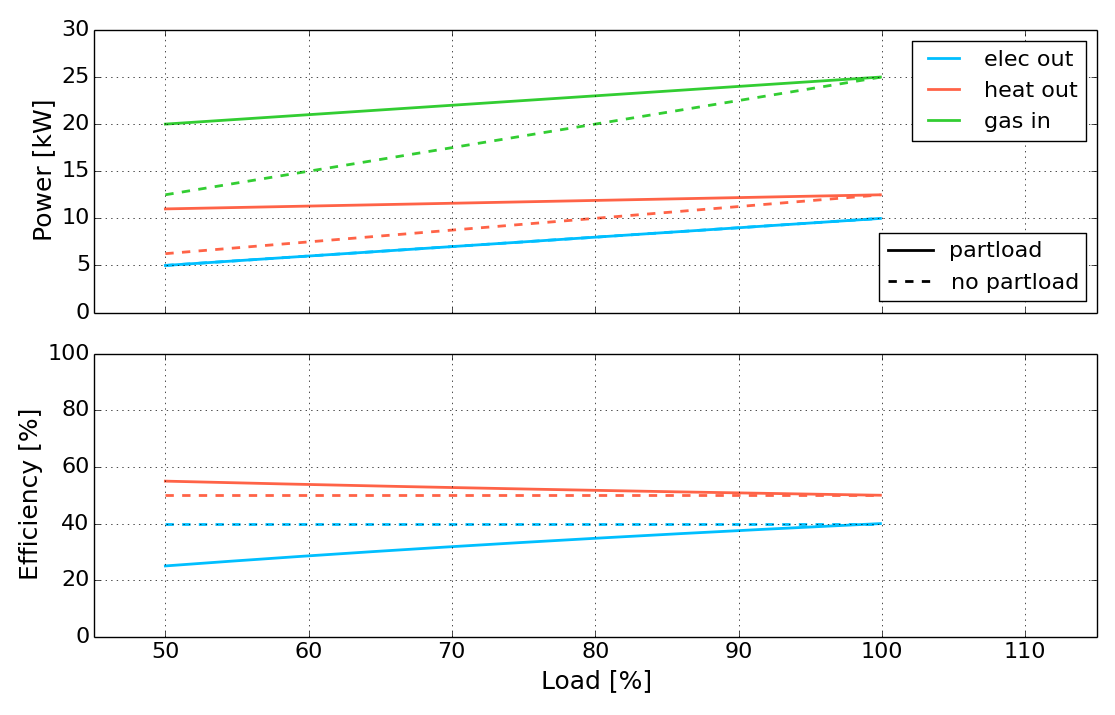
So with setting the ratios for full load and minimum part-load we defined the part-load performance curve of our process. Points between full load and minimum part-load are approximated as a linear function between them. (Note: If Partload in MIP-Settings is set to False, part-load behaviour is not considered and the efficiencies defined by ratio are constant for all operating points. The values in ratio-partload are ignored).

The following figure shows the power inputs/outputs and efficiencies of a 10 kW (elec!) chp unit with the parameters used in this example with and without considering part-load behaviour.

Edit Example:

Delete all existing processes and add the new processes chp, wind_1, wind_2 and boiler. Set the ratios as shown in the table. Because part-load behaviour is not considered in this example, we just use the same values for ratio-partload (we could leave the ratio-partload column empty or set to any arbitrary value as long as Partload in MIP-Equations is deactivated)

Sheet Process-Commodity

Process	Commodity	Direction	ratio	ratio-partload
chp	gas	In	2.50	2.50
chp	elec	Out	1.00	1.00
chp	heat	Out	1.25	1.25
wind_1	wind1	In	1.00	1.00
wind_1	elec	Out	1.00	1.00
wind_2	wind2	In	1.00	1.00
wind_2	elec	Out	1.00	1.00
boiler	gas	In	1.10	1.10
boiler	heat	Out	1.00	1.00

Process Class

Define a Process Class and add fees/subsidies for a produced/consumed commodity or capacity and energy limits for this class.

Processes can be assigned to a process class in the columns class in the Process sheet (See Process_ref). Make sure you use exactly the same names.

• Class: Name of the Process Class
• Commodity: Commodity of the processes within the class
• Direction: Direction of the commodity within the processes of this class (In or Out)
• fee: additional fee for produced/consumed energy in this class. (Positive values: Pay Money; Negative Values: Receive Money)
• cap-max: Maximum value for the sum of all process capacities of this class (Independent from Commodity)
• energy-max: Maximum value for the sum of energy of the specified commodity that can be produced/consumed by the class within one year

Edit Example:

Delete all existing processes classes and add the new classes CHP and WIND with Commodity elec and Direction Out. Set the ratios as shown in the table. This sets a maximum of 20000 kW for the total capacity of wind turbines, a subsidy of 0.05 Euro/kWh for produced electricity of the wind turbines (weather sold to the grid or used to cover the demand) and a fee of 0.02 Euro/kWh for produced electricity out of our chp unit.

Sheet Process-Class

Class	Commodity Direction	fee	cap-max	energy-max
CHP	elec	Out	0.02	inf	inf
WIND	elec	Out	-0.05	20000	inf

Storage

Define storages for a commodity with technical parameters and specific costs.

• Storage: Name of storage
• Commodity: Commodity that can be stored
• Num: Number of identical storages
• cost-inv-p: Specific investment costs for new charge/discharge power capacities of storage (in Euro/kW)
• cost-inv-e: Specific investment costs for new energy capacities of storage (in Euro/kWh).
• cost-fix-p: Specific annual fix costs per installed charge/discharge power (in Euro/kW/a)
• cost-fix-e: Specific annual fix costs per installed energy (in Euro/kWh/a)
• cost-var: Specific variable costs per energy throughput (in Euro/kWh)
• cap-installed-p: Already installed charge/discharge power capacity of storage (no additional investment costs) (in kW)
• cap-new-min-p: Minimum charge/discharge power capacity of storage to be build, if process is built. It is always possible that the storage isn’t built at all. (in kW) (Note: only considered if Min-Cap in MIP-Settings is True)
• cap-new-max-p: Maximum new charge/discharge power capacity of storage (in kW)
• cap-installed-e:Already installed energy capacity of storage (no additional investment costs) (in kWh)
• cap-new-min-e: Minimum power capacity of storage to be build, if process is built. It is always possible that the storage isn’t built at all. (in kWh) (Note: only considered if Min-Cap in MIP-Settings is True)
• cap-new-max-e: Maximum new energy capacity of storage (in kWh)
• max-p-e-ratio: Maximum relation of charge-discharge power to storage energy (in kW/kWh). power <= energy * ratio
• eff-in: Charge efficiency (in %/100)
• eff-out: Discharge efficiency (in %/100)
• self-discharge: Self discharge of storage (in %/h/100)
• cycles-max: Maximum number of full cycles before end of life of storage
• DOD: Depth of discharge. Usable share of energy of storage (in %/100)
• initial-soc: Initial state of charge of the storage (in %/100).
• depreciation: Depreciation period. Economic lifetime (more conservative than technical lifetime) of a process investment in years (a). Used to calculate annuity factor for investment costs.
• wacc: Weighted average cost of capital. Percentage (%/100) of costs for capital after taxes. Used to calculate annuity factor for investment costs.

Note: All values for the storage energy capacities and energy specific costs are related to the energy that can be stored in the storage with 100 % depth of discharge (DOD). The energy that can be used out of the storage might be less, depending on the DOD and the discharge efficiency eff-out.

Edit Example:

Change the parameters of the storage battery and heat storage as shown in the table.

Sheet Storage (1/3)

Storage	Commodity	Num	cost-inv-p	cost-inv-e	cost-fix-p	cost-fix-e	cost-var
battery elec	1	0	1000	0	0	0
heat storage	heat	1	0	10	0	0	0

Sheet Storage (2/3)

Storage	Commodity	Num	cap-installed-p	cap-new-min-p	cap-new-max-p	cap-installed-e	cap-new-min-e	cap-new-max-e	max-p-e-ratio
battery	elec	1	0	0	1e6	0	0	100000	2
heat storage	heat	1	0	0	1e6	0	0	30000	1

Sheet Storage (3/3)

Storage	Commodity	Num	eff-in	eff-out	self-discharge	cycles-max	DOD	initial-soc	depreciation	wacc
battery	elec	1	0.900	0.900	0.0001	10000	1	0	10	0.05
heat storage	heat	1	0.950	0.950	0.0001	1000000	1	0	10	0.05

Demand

Time-series: (average) power demand for every commodity to be satisfied for every time-step (in kW).

Edit Example:

Keep the demand time-series for elec and heat as they are

Sheet Demand

Time	elec	heat
1	28749.52	8856
2	29383.66	8676
3	29496.09	9104
4	29592.54	8892
5	30346.42	8764
6	31300.91	8560
7	…	…

SupIm

Intermittent Supply: A time-series normalised to a maximum value of 1 relative to the installed capacity of a process using this commodity as input. For example, a wind power time-series should reach value 1, when the wind speed exceeds the modelled wind turbine’s design wind speed is exceeded. This implies that any non-linear behaviour of intermittent processes can already be incorporated while preparing this time-series.

Edit Example:

Copy the intermittent supply timeseries wind1 and wind2 from intermittent_supply_wind.xlsx to the SupIm sheet.

Sheet SupIm

Time	wind1	wind2
1	0.91	1.00
2	1.00	1.00
3	1.00	1.00
4	1.00	1.00
5	1.00	1.00
6	0.88	1.00
7	…	…

Note

For reference, this is how NewFactory.xlsx and NewFactory.xlsm look for me having performed the above steps.

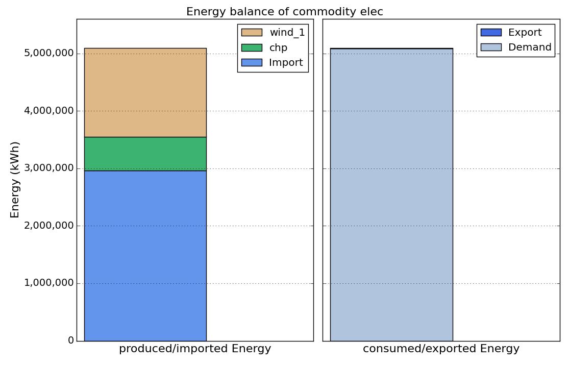
Test-drive the input

Now that NewFactory.xlsx or NewFactory.xlsm is ready to go, run the model:

run-excel-ref or Run from Python

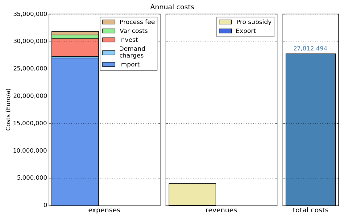
Th obtained results should look like this:

MIP-Equations

This sections shows the influence of the equations that can be activated/deactivated in the sheet MIP-Equations with the help of an example.

See MIP-Equations for a short Description.

Storage In-Out

If activated, a constrained is added, that prevents storages from charging and discharging one commodity at the same time.

Open NewFactory.xlsx or NewFactory.xlsm, change the costs for gas import from 0.05 Euro/kWh to 0.03 Euro/kWh.

Sheet Ext-Import

Time	elec	gas
1	0.15	0.03
2	0.15	0.03
3	0.15*	0.03
4	0.15	0.03
5	0.15	0.03
6	0.15	0.03
7	…	…

Save the new file and run the model. Take a look at the heat time-series result figure:

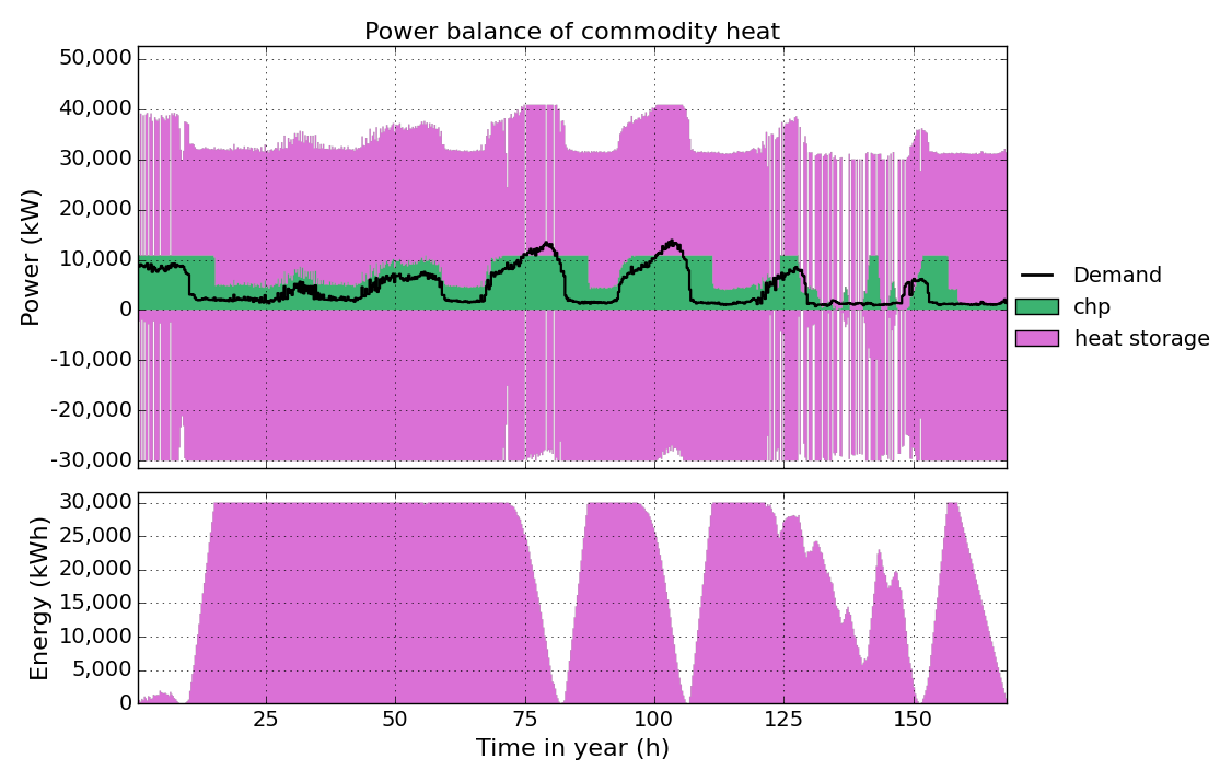
As you can see the heat storage is charged and discharged at the same time for almost the whole period. This is because of the low gas costs producing electricity from the chp unit becomes much cheaper than importing it from the grid. The model tries to produce as much electricity from the chp unit as possible, but is limited because of the lower heat demand (the produced heat has to be consumed as well). The model equations do not allow dumping energy. So to get rid of the heat produced, th model uses the heat storage efficiency to generate losses by simply charging and discharging at the same time.

To avoid this, activate Storage In-Out in the sheet MIP-Equations:

Sheet MIP-Equations

Equation	Active
Storage In-Out	yes
Partload	no
Min-Cap	no

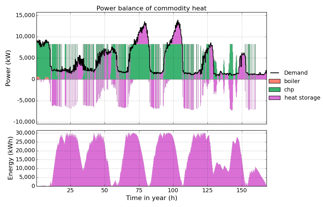
Run the model again. This will take a little more time than before, because the equation uses an integer variable and the model becomes a mixed integer linear optimisation problem. Looking at the heat time-series result figure again, you can see that charging/discharging of the storage at the same time is avoided now.

Partload

If activated, minimum part-load settings, part-load efficiencies as well as start-up costs of processes are considered.

Open NewFactory.xlsx or NewFactory.xlsm.

To reduce computation time, we assume that we already have a chp unit with a capacity of 7,000 kW in our factory and do not allow to build more capacity for this process. Therefore we change the parameters cap-installed and cap-new-max in the Process sheet as shown in the table below.

Sheet Process

Process	Num	…	cap-installed	cap-new-min	cap-new-max	partload-min	start-up-energy	…
chp	1	…	7000	0	0	0	0	…
wind_1	1	…	0	0	1e6	0	0	…
wind_2	1	…	0	0	1e6	0	0	…
boiler	1	…	0	0	1e6	0	0	…

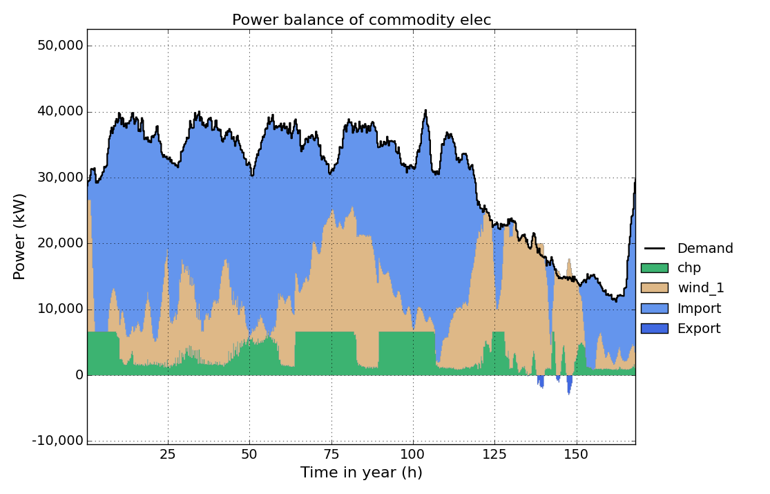
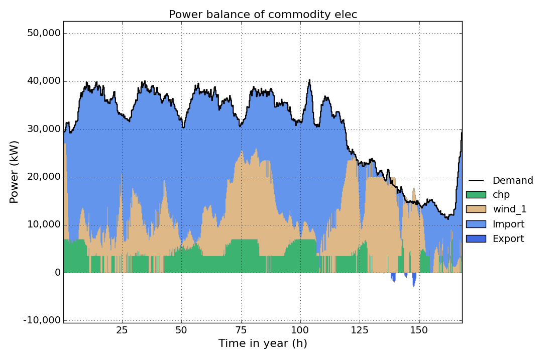
Save the input file, run the model and take a look at the elec timeseries result figure.

Now we want to implement a minimum partload for the chp unit. Therefore we set the parameter partload-min for the chp unit in the Process sheet to 0.5. That means, if the chp unit is running, it has to run at minimum 50% of its rated (installed) power.

Sheet Process

Process	Num	…	cap-installed	cap-new-min	cap-new-max	partload-min	start-up-energy	…
chp	1	…	7000	0	0	0.5	0	…
wind_1	1	…	0	0	1e6	0	0	…
wind_2	1	…	0	0	1e6	0	0	…
boiler	1	…	0	0	1e6	0	0	…

To activate this constrained , we have to activate Partload in the sheet MIP-Equations.

Sheet MIP-Equations

Equation	Active
Storage In-Out	no
Partload	yes
Min-Cap	no

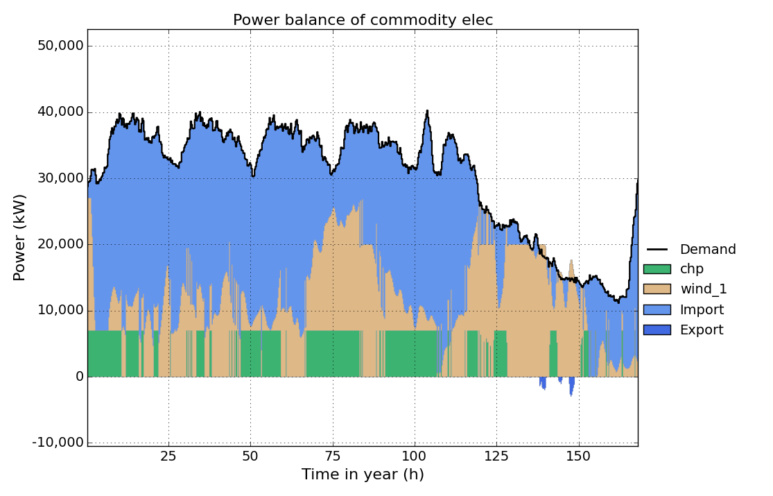
Now run the model and take a look at the elec time-series result figure again. You can see that the electric power output of the chp now is always greater than 50% of the installed capacity (7000 kW), when the chp unit is running.

In the next step we want to see the influence of considering part-load efficiency. Therefore we change the ratio-partload values in the Process-Commodity sheet as shown below , without changing the values in Process sheet. With this changes the chp unit has an electric (thermal) efficiency of 40% (50%) at full load and 30% (55%) at minimum part-load (50% of max. power). See Process-Commodity for detailed information. (Note: part-load efficiency can only be considered if partload-min is greater than zero.)

Sheet Process

Process	Num	…	cap-installed	cap-new-min	cap-new-max	partload-min	start-up-energy	…
chp	1	…	7000	0	0	0.5	0	…
wind_1	1	…	0	0	1e6	0	0	…
wind_2	1	…	0	0	1e6	0	0	…
boiler	1	…	0	0	1e6	0	0	…

Sheet Process-Commodity

Process	Commodity	Direction	ratio	ratio-partload
chp	gas	In	2.50	4.00
chp	elec	Out	1.00	1.00
chp	heat	Out	1.25	2.2

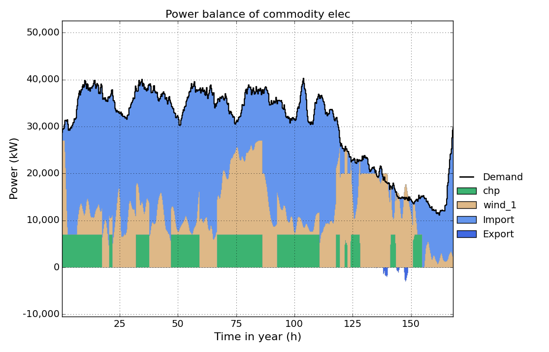
Run the model and take a look at the elec time-series result figure again. You can see how the model tries to run the chp unit at full load as much as possible to benefit from it’s better electric efficiency at full load and reduce costs for gas import.

In the last step we add start-up costs for the chp unit, by setting the parameter start-up-energy in the Process sheet to 0.1 kWh/kW. This means, that for every start-up all input commodities (here gas) consume 0.1 kWh * ratio (here 0.1*2.5 kWh) per installed capacity of the process. (**Note:**Start-up costs only occur, if partload-min is greater than zero.

Sheet Process

Process	Num	…	cap-installed	cap-new-min	cap-new-max	partload-min	start-up-energy	…
chp	1	…	7000	0	0	0.5	0.1	…
wind_1	1	…	0	0	1e6	0	0	…
wind_2	1	…	0	0	1e6	0	0	…
boiler	1	…	0	0	1e6	0	0	…

Run the model and take a look at the elec time-series result figure again. You can see how the number of start-up’s is reduced to minimize start-up costs.

Min-Cap

Consider minimal installed capacities of processes and storages if activated. This allows to set a minimum capacity of processes and storages, that has to be build, if the process is built at all (it still can not be built at all). Setting minimal and maximal capacities of processes/storages to the same level, this allows investigating if building a specific process/storage with a specific size is cost efficient.

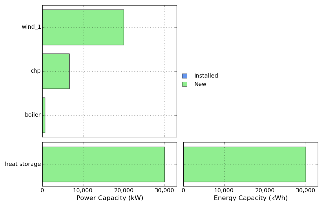
Open and run NewFactory.xlsx or NewFactory.xlsm, and take a look at the capacities result figure:

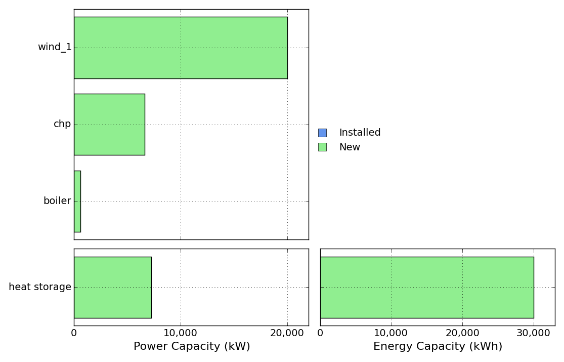
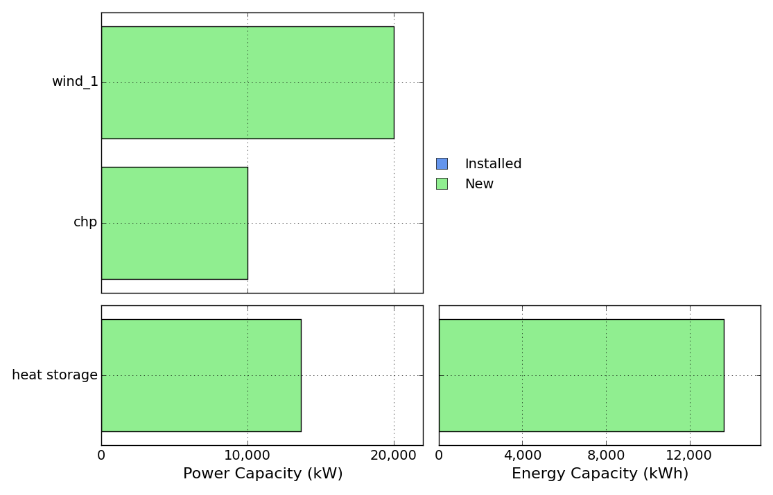
Now we want to know, if a chp unit with exactly 10,000 kW is cost-efficient for our factory. Therefore we change the cap-new-min and the cap-new-max parameter in the Process sheet to 10,000 kW.

Sheet Process

Process	Num	…	cap-installed	cap-new-min	cap-new-max	…
chp	1	…	0	10000	10000	…
wind_1	1	…	0	0	1e6	…
wind_2	1	…	0	0	1e6	…
boiler	1	…	0	0	1e6	…

To activate this constraint , we have to activate Min-Cap in the sheet MIP-Equations.

Sheet MIP-Equations

Equation	Active
Storage In-Out	no
Partload	yes
Min-Cap	no

Running the file with the above changes show the following capacities result figure, You can see, that a chp unit with exactly 10,000 kW is built.